Using Databases and SQL

What is a database?

A database is a file that is organized for storing data. Most databases are organized like a dictionary in the sense that they map from keys to values. The biggest difference is that the database is on disk (or other permanent storage), so it persists after the program ends. Because a database is stored on permanent storage, it can store far more data than a dictionary, which is limited to the size of the memory in the computer.

Like a dictionary, database software is designed to keep the inserting and accessing of data very fast, even for large amounts of data. Database software maintains its performance by building indexes as data is added to the database to allow the computer to jump quickly to a particular entry.

There are many different database systems which are used for a wide variety of purposes including: Oracle, MySQL, Microsoft SQL Server, PostgreSQL, and SQLite. We focus on SQLite in this book because it is a very common database and is already built into Python. SQLite is designed to be embedded into other applications to provide database support within the application. For example, the Firefox browser also uses the SQLite database internally as do many other products.

http://sqlite.org/

SQLite is well suited to some of the data manipulation problems that we see in Informatics.

Database concepts

When you first look at a database it looks like a spreadsheet with multiple sheets. The primary data structures in a database are: tables, rows, and columns.

In technical descriptions of relational databases the concepts of table, row, and column are more formally referred to as relation, tuple, and attribute, respectively. We will use the less formal terms in this chapter.

Database Browser for SQLite

While this chapter will focus on using Python to work with data in SQLite database files, many operations can be done more conveniently using software called the Database Browser for SQLite which is freely available from:

http://sqlitebrowser.org/

Using the browser you can easily create tables, insert data, edit data, or run simple SQL queries on the data in the database.

In a sense, the database browser is similar to a text editor when working with text files. When you want to do one or very few operations on a text file, you can just open it in a text editor and make the changes you want. When you have many changes that you need to do to a text file, often you will write a simple Python program. You will find the same pattern when working with databases. You will do simple operations in the database manager and more complex operations will be most conveniently done in Python.

Creating a database table

Databases require more defined structure than Python lists or dictionaries¹.

When we create a database table we must tell the database in advance the names of each of the columns in the table and the type of data which we are planning to store in each column. When the database software knows the type of data in each column, it can choose the most efficient way to store and look up the data based on the type of data.

You can look at the various data types supported by SQLite at the following url:

http://www.sqlite.org/datatypes.html

Defining structure for your data up front may seem inconvenient at the beginning, but the payoff is fast access to your data even when the database contains a large amount of data.

The code to create a database file and a table named Track with two columns in the database is as follows:

import sqlite3

conn = sqlite3.connect('music.sqlite')
cur = conn.cursor()

cur.execute('DROP TABLE IF EXISTS Track')
cur.execute('CREATE TABLE Track (title TEXT, plays INTEGER)')

conn.close()

# Code: https://www.py4e.com/code3/db1.py

The connect operation makes a “connection” to the database stored in the file music.sqlite in the current directory. If the file does not exist, it will be created. The reason this is called a “connection” is that sometimes the database is stored on a separate “database server” from the server on which we are running our application. In our simple examples the database will just be a local file in the same directory as the Python code we are running.

A cursor is like a file handle that we can use to perform operations on the data stored in the database. Calling cursor() is very similar conceptually to calling open() when dealing with text files.

Once we have the cursor, we can begin to execute commands on the contents of the database using the execute() method.

Database commands are expressed in a special language that has been standardized across many different database vendors to allow us to learn a single database language. The database language is called Structured Query Language or SQL for short.

http://en.wikipedia.org/wiki/SQL

In our example, we are executing two SQL commands in our database. As a convention, we will show the SQL keywords in uppercase and the parts of the command that we are adding (such as the table and column names) will be shown in lowercase.

The first SQL command removes the Track table from the database if it exists. This pattern is simply to allow us to run the same program to create the Track table over and over again without causing an error. Note that the DROP TABLE command deletes the table and all of its contents from the database (i.e., there is no “undo”).

cur.execute('DROP TABLE IF EXISTS Track ')

The second command creates a table named Track with a text column named title and an integer column named plays.

cur.execute('CREATE TABLE Track (title TEXT, plays INTEGER)')

Now that we have created a table named Track, we can put some data into that table using the SQL INSERT operation. Again, we begin by making a connection to the database and obtaining the cursor. We can then execute SQL commands using the cursor.

The SQL INSERT command indicates which table we are using and then defines a new row by listing the fields we want to include (title, plays) followed by the VALUES we want placed in the new row. We specify the values as question marks (?, ?) to indicate that the actual values are passed in as a tuple ( 'My Way', 15 ) as the second parameter to the execute() call.

import sqlite3

conn = sqlite3.connect('music.sqlite')
cur = conn.cursor()

cur.execute('INSERT INTO Track (title, plays) VALUES (?, ?)',
    ('Thunderstruck', 20))
cur.execute('INSERT INTO Track (title, plays) VALUES (?, ?)',
    ('My Way', 15))
conn.commit()

print('Track:')
cur.execute('SELECT title, plays FROM Track')
for row in cur:
     print(row)

cur.execute('DELETE FROM Track WHERE plays < 100')
conn.commit()

cur.close()

# Code: https://www.py4e.com/code3/db2.py

First we INSERT two rows into our table and use commit() to force the data to be written to the database file.

Then we use the SELECT command to retrieve the rows we just inserted from the table. On the SELECT command, we indicate which columns we would like (title, plays) and indicate which table we want to retrieve the data from. After we execute the SELECT statement, the cursor is something we can loop through in a for statement. For efficiency, the cursor does not read all of the data from the database when we execute the SELECT statement. Instead, the data is read on demand as we loop through the rows in the for statement.

The output of the program is as follows:

Track:
('Thunderstruck', 20)
('My Way', 15)

Our for loop finds two rows, and each row is a Python tuple with the first value as the title and the second value as the number of plays.

At the very end of the program, we execute an SQL command to DELETE the rows we have just created so we can run the program over and over. The DELETE command shows the use of a WHERE clause that allows us to express a selection criterion so that we can ask the database to apply the command to only the rows that match the criterion. In this example the criterion happens to apply to all the rows so we empty the table out so we can run the program repeatedly. After the DELETE is performed, we also call commit() to force the data to be removed from the database.

Structured Query Language summary

So far, we have been using the Structured Query Language in our Python examples and have covered many of the basics of the SQL commands. In this section, we look at the SQL language in particular and give an overview of SQL syntax.

Since there are so many different database vendors, the Structured Query Language (SQL) was standardized so we could communicate in a portable manner to database systems from multiple vendors.

A relational database is made up of tables, rows, and columns. The columns generally have a type such as text, numeric, or date data. When we create a table, we indicate the names and types of the columns:

CREATE TABLE Track (title TEXT, plays INTEGER)

To insert a row into a table, we use the SQL INSERT command:

INSERT INTO Track (title, plays) VALUES ('My Way', 15)

The INSERT statement specifies the table name, then a list of the fields/columns that you would like to set in the new row, and then the keyword VALUES and a list of corresponding values for each of the fields.

The SQL SELECT command is used to retrieve rows and columns from a database. The SELECT statement lets you specify which columns you would like to retrieve as well as a WHERE clause to select which rows you would like to see. It also allows an optional ORDER BY clause to control the sorting of the returned rows.

SELECT * FROM Track WHERE title = 'My Way'

Using * indicates that you want the database to return all of the columns for each row that matches the WHERE clause.

Note, unlike in Python, in a SQL WHERE clause we use a single equal sign to indicate a test for equality rather than a double equal sign. Other logical operations allowed in a WHERE clause include <, >, <=, >=, !=, as well as AND and OR and parentheses to build your logical expressions.

You can request that the returned rows be sorted by one of the fields as follows:

SELECT title,plays FROM Track ORDER BY title

It is possible to UPDATE a column or columns within one or more rows in a table using the SQL UPDATE statement as follows:

UPDATE Track SET plays = 16 WHERE title = 'My Way'

The UPDATE statement specifies a table and then a list of fields and values to change after the SET keyword and then an optional WHERE clause to select the rows that are to be updated. A single UPDATE statement will change all of the rows that match the WHERE clause. If a WHERE clause is not specified, it performs the UPDATE on all of the rows in the table.

To remove a row, you need a WHERE clause on an SQL DELETE statement. The WHERE clause determines which rows are to be deleted:

DELETE FROM Track WHERE title = 'My Way'

These four basic SQL commands (INSERT, SELECT, UPDATE, and DELETE) allow the four basic operations needed to create and maintain data. We use “CRUD” (Create, Read, Update, and Delete) to capture all these concepts in a single term.²

Multiple tables and basic data modeling

The real power of a relational database is when we create multiple tables and make links between those tables. The act of deciding how to break up your application data into multiple tables and establishing the relationships between the tables is called data modeling. The design document that shows the tables and their relationships is called a data model.

Data modeling is a relatively sophisticated skill and we will only introduce the most basic concepts of relational data modeling in this section. For more detail on data modeling you can start with:

http://en.wikipedia.org/wiki/Relational_model

Lets say for our tracks database we wanted to track the name of the artist for each track in addition to the title and number of plays for each track. A simple approach might be to simply add another column to the database called artist and put the name of the artist in the column as follows:

DROP TABLE IF EXISTS Track;
CREATE TABLE Track (title TEXT, plays INTEGER, artist TEXT);

Then we could insert a few tracks into our table.

INSERT INTO Track (title, plays, artist)
    VALUES ('My Way', 15, 'Frank Sinatra');
INSERT INTO Track (title, plays, artist)
    VALUES ('New York', 25, 'Frank Sinatra');

If we were to look at our data with a SELECT * FROM Track statement, it looks like we have done a fine job.

sqlite> SELECT * FROM Track;
My Way|15|Frank Sinatra
New York|25|Frank Sinatra
sqlite>

We have made a very bad error in our data modeling. We have violated the rules of database normalization.

https://en.wikipedia.org/wiki/Database_normalization

While database normalization seems very complex on the surface and contains a lot of mathematical justifications, for now we can reduce it all into one simple rule that we will follow.

We should never put the same string data in a column more than once. If we need the data more than once, we create a numeric key for the data and reference the actual data using this key. Especially if the multiple entries refer to the same object.

To demonstrate the slippery slope we are going down by assigning string columns to out database model, think about how we would change the data model if we wanted to keep track of the eye color of our artists? Would we do this?

DROP TABLE IF EXISTS Track;
CREATE TABLE Track (title TEXT, plays INTEGER,
    artist TEXT, eyes TEXT);
INSERT INTO Track (title, plays, artist, eyes)
    VALUES ('My Way', 15, 'Frank Sinatra', 'Blue');
INSERT INTO Track (title, plays, artist, eyes)
    VALUES ('New York', 25, 'Frank Sinatra', 'Blue');

Since Frank Sinatra recorded over 1200 songs, are we really going to put the string ‘Blue’ in 1200 rows in our Track table. And what would happen if we decided his eye color was ‘Light Blue’? Something just does not feel right.

The correct solution is to create a table for the each Artist and store all the data about the artist in that table. And then somehow we need to make a connection between a row in the Track table to a row in the Artist table. Perhaps we could call this “link” between two “tables” a “relationship” between two tables. And that is exactly what database experts decided to all these links.

Lets make an Artist table as follows:

DROP TABLE IF EXISTS Artist;
CREATE TABLE Artist (name TEXT, eyes TEXT);
INSERT INTO Artist (name, eyes)
   VALUES ('Frank Sinatra', 'blue');

Now we have two tables but we need a way to link rows in the two tables. To do this, we need why we call ‘keys’. These keys will just be integer numbers that we can use to lookup a row in different table. If we are going to make links to rows inside of a table, we need to add a primary key to the rows in the table. By convention we usually name the primary key column ‘id’. So our Artist table looks as follows:

DROP TABLE IF EXISTS Artist;
CREATE TABLE Artist (id INTEGER, name TEXT, eyes TEXT);
INSERT INTO Artist (id, name, eyes)
   VALUES (42, 'Frank Sinatra', 'blue');

Now we have a row in the table for ‘Frank Sinatra’ (and his eye color) and a primary key of ‘42’ to use to link our tracks to him. So we alter our Track table as follows:

DROP TABLE IF EXISTS Track;
CREATE TABLE Track (title TEXT, plays INTEGER,
    artist_id INTEGER);
INSERT INTO Track (title, plays, artist_id)
    VALUES ('My Way', 15, 42);
INSERT INTO Track (title, plays, artist_id)
    VALUES ('New York', 25, 42);

The artist_id column is an integer, and by naming convention is a foreign key pointing at a primary key in the Artist table. We call it a foreign key because it is pointing to a row in a different table.

Now we are following the rules of database normalization, but when we want to get data out of our database, we don’t want to see the 42, we want to see the name and eye color of the artist. To do this we use the JOIN keyword in our SELECT statement.

SELECT title, plays, name, eyes
FROM Track JOIN Artist
ON Track.artist_id = Artist.id;

The JOIN clause includes an ON condition that defines how the rows are to to be connected. For each row in Track add the data from Artist from the row where artist_id Track table matches the id from the Artist table.

The output would be:

My Way|15|Frank Sinatra|blue
New York|25|Frank Sinatra|blue

While it might seem a little clunky and your instincts might tell you that it would be faster just to keep the data in one table, it turns out the the limit on database performance is how much data needs to be scanned when retrieving a query. While they details are very complex, integers are a lot smaller than strings (especially Unicode) and far quicker to to move and compare.

Data model diagrams

While our Track and Artist database design is simple with just two tables and a single one-to-many relationship, these data models can get complicated quickly and are easier to understand if we can make a graphical representation of our data model.

A Verbose One-to-Many Data Model\label{figvrbo2m} — A Verbose One-to-Many Data Model

While there are many graphical representations of data models, we will use one of the “classic” appraches, called “Crow’s Foot Diagrams” as shown in Figure . Each table is shown as a box with the name of the table and its columns. Then where there is a relationship between two tables a line is drawn connecting the tables with a notation added to the end of each line indicating the nature of the relationship.

https://en.wikipedia.org/wiki/Entity-relationship_model

In this case, “many” tracks can be associated with each artist. So the track end is shown with the crow’s foot spread out indicating it is the” “many” end. The artist end is shown with a vertical like that indicates “one”. There will be “many” artists in general, but the important aspect is that for each artist there will be many tracks. And each of those artists may be associated with multiple tracks.

You will note that the column that holds the foreign_key like artist_id is on the “many” end and the primary key is at the “one” end.

Since the pattern of foreign and primary key placement is so consistent and follows the “many” and “one” ends of the lines, we never include either the primary or foreign key columns in our diagram of the data model as shown in the second diagram as shown in Figure . The columns are thought of as “implementation detail” to capture the nature of the relationship details and not an essential part of the data being modeled.

A Succinct One-to-Many Data Model\label{figo2m} — A Succinct One-to-Many Data Model

Automatically creating primary keys

In the above example, we arbitrarily assigned Frank the primary key of 42. However when we are inserting millions or rows, it is nice to have the database automatically generate the values for the id column. We do this by declaring the id column as a PRIMARY KEY and leave out the id value when inserting the row:

DROP TABLE IF EXISTS Artist;
CREATE TABLE Artist (id INTEGER PRIMARY KEY,
    name TEXT, eyes TEXT);
INSERT INTO Artist (name, eyes)
   VALUES ('Frank Sinatra', 'blue');

Now we have instructed the database to auto-assign us a unique value to the Frank Sinatra row. But we then need a way to have the database tell us the id value for the recently inserted row. One way is to use a SELECT statement to retrieve data from an SQLite built-in-fuction called last_insert_rowid().

sqlite> DROP TABLE IF EXISTS Artist;
sqlite> CREATE TABLE Artist (id INTEGER PRIMARY KEY,
   ...>     name TEXT, eyes TEXT);
sqlite> INSERT INTO Artist (name, eyes)
   ...>    VALUES ('Frank Sinatra', 'blue');
sqlite> select last_insert_rowid();
1
sqlite> SELECT * FROM Artist;
1|Frank Sinatra|blue
sqlite>

Once we know the id of our ‘Frank Sinatra’ row, we can use it when we INSERT the tracks into the Track table. As a general strategy, we add these id columns to any table we create:

sqlite> DROP TABLE IF EXISTS Track;
sqlite> CREATE TABLE Track (id INTEGER PRIMARY KEY,
   ...>     title TEXT, plays INTEGER, artist_id INTEGER);

Note that the artist_id value is the new auto-assigned row in the Artist table and that while we added an INTEGER PRIMARY KEY to the the Track table, we did not include id in the list of fields on the INSERT statements into the Track table. Again this tells the database to choose a unique value for us for the id column.

sqlite> INSERT INTO Track (title, plays, artist_id)
   ...>     VALUES ('My Way', 15, 1);
sqlite> select last_insert_rowid();
1
sqlite> INSERT INTO Track (title, plays, artist_id)
   ...>     VALUES ('New York', 25, 1);
sqlite> select last_insert_rowid();
2
sqlite>

You can call SELECT last_insert_rowid(); after each of the inserts to retrieve the value that the database assigned to the id of each newly created row. Later when we are coding in Python, we can ask for the id value in our code and store it in a variable for later use.

Logical keys for fast lookup

If we had a table full of artists and a table full of tracks, each with a foreign key link to a row in a table full of artists and we wanted to list all the tracks that were sung by ‘Frank Sinatra’ as follows:

SELECT title, plays, name, eyes
FROM Track JOIN Artist
ON Track.artist_id = Artist.id
WHERE Artist.name = 'Frank Sinatra';

Since we have two tables and a foreign key between the two tables, our data is well-modeled, but if we are going to have millions of records in the Artist table and going to do a lot of lookups by artist name, we would benefit if we gave the database a hint about our intended use of the name column.

We do this by adding an “index” to a text column that we intend to use in WHERE clauses:

CREATE INDEX artist_name ON Artist(name);

When the database has been told that an index is needed on a column in a table, it stores extra information to make it possible to look up a row more quickly using the indexed field (name in this example). Once you request that an index be created, there is nothing special that is needed in the SQL to access the table. The database keeps the index up to date as data is inserted, deleted, and updated, and uses it automatically if it will increase the performance of a database query.

These text columns that are used to find rows based on some information in the “real world” like the name of an artist are called Logical keys.

Adding constraints to the data database

We can also use an index to enforce a constraint (i.e. rules) on our database operations. The most common constraint is a uniqueness constraint which insists that all of the values in a column are unique. We can add the optional UNIQUE keyword, to the CREATE INDEX statement to tell the database that we would like it to enforce the constraint on our SQL. We can drop and re-create the artist_name index with a UNIQUE constraint as follows.

DROP INDEX artist_name;
CREATE UNIQUE INDEX artist_name ON Artist(name);

If we try to insert ‘Frank Sinatra’ a second time, it will fail with an error.

sqlite> SELECT * FROM Artist;
1|Frank Sinatra|blue
sqlite> INSERT INTO Artist (name, eyes)
   ...>    VALUES ('Frank Sinatra', 'blue');
Runtime error: UNIQUE constraint failed: Artist.name (19)
sqlite>

We can tell the database to ignore any duplicate key errors by adding the IGNORE keyword to the INSERT statement as follows:

sqlite> INSERT OR IGNORE INTO Artist (name, eyes)
   ...>     VALUES ('Frank Sinatra', 'blue');
sqlite> SELECT id FROM Artist WHERE name='Frank Sinatra';
1
sqlite>

By combining an INSERT OR IGNORE and a SELECT we can insert a new record if the name is not already there and whether or not the record is already there, retrieve the primary key of the record.

sqlite> INSERT OR IGNORE INTO Artist (name, eyes)
   ...>      VALUES ('Elvis', 'blue');
sqlite> SELECT id FROM Artist WHERE name='Elvis';
2
sqlite> SELECT * FROM Artist;
1|Frank Sinatra|blue
2|Elvis|blue
sqlite>

Since we have not added a uniqueness constraint to the eye color column, there is no problem having multiple ‘Blue’ values in the eye column.

Tracks, Albums, and Artists\label{figtaa} — Tracks, Albums, and Artists

Sample multi-table application

A sample application called tracks_csv.py shows how these ideas can be combined to parse textual data and load it into several tables using a proper data model with relational connections between the tables.

This application reads and parses a comma-separated file tracks.csv based on an export from Dr. Chuck’s iTunes library.

Another One Bites The Dust,Queen,Greatest Hits,55,100,217103
Asche Zu Asche,Rammstein,Herzeleid,79,100,231810
Beauty School Dropout,Various,Grease,48,100,239960
Black Dog,Led Zeppelin,IV,109,100,296620
...

The columns in this file are: title, artist, album, number of plays, rating (0-100) and length in milliseconds.

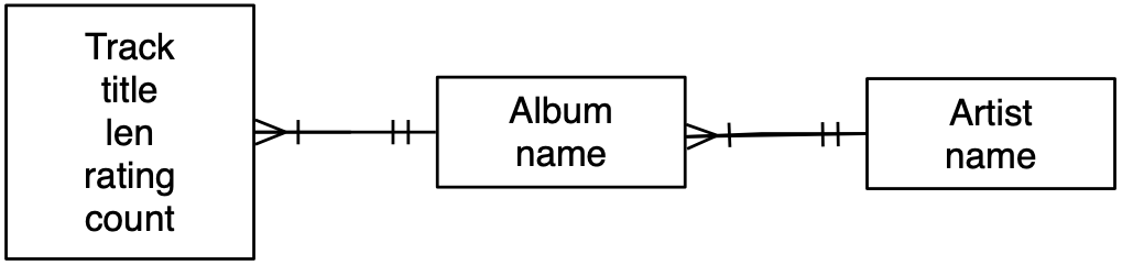
Our data model is shown in Figure and described in SQL as follows:

DROP TABLE IF EXISTS Artist;
DROP TABLE IF EXISTS Album;
DROP TABLE IF EXISTS Track;

CREATE TABLE Artist (
    id INTEGER PRIMARY KEY,
    name TEXT UNIQUE
);

CREATE TABLE Album (
    id INTEGER PRIMARY KEY,
    artist_id  INTEGER,
    title TEXT UNIQUE
);

CREATE TABLE Track (
    id INTEGER PRIMARY KEY,
    title TEXT UNIQUE,
    album_id INTEGER,
    len INTEGER, rating INTEGER, count INTEGER
);

We are adding the UNIQUE keyword to TEXT columns that we would like to have a uniqueness constraint that we will use in INSERT IGNORE statements. This is more succinct that separate CREATE INDEX statements but has the same effect.

With these tables in place, we write the following code tracks_csv.py to parse the data and insert it into the tables:

import sqlite3

conn = sqlite3.connect('trackdb.sqlite')
cur = conn.cursor()

handle = open('tracks.csv')

for line in handle:
    line = line.strip();
    pieces = line.split(',')
    if len(pieces) != 6 : continue

    name = pieces[0]
    artist = pieces[1]
    album = pieces[2]
    count = pieces[3]
    rating = pieces[4]
    length = pieces[5]

    print(name, artist, album, count, rating, length)

    cur.execute('''INSERT OR IGNORE INTO Artist (name)
        VALUES ( ? )''', ( artist, ) )
    cur.execute('SELECT id FROM Artist WHERE name = ? ', (artist, ))
    artist_id = cur.fetchone()[0]

    cur.execute('''INSERT OR IGNORE INTO Album (title, artist_id)
        VALUES ( ?, ? )''', ( album, artist_id ) )
    cur.execute('SELECT id FROM Album WHERE title = ? ', (album, ))
    album_id = cur.fetchone()[0]

    cur.execute('''INSERT OR REPLACE INTO Track
        (title, album_id, len, rating, count)
        VALUES ( ?, ?, ?, ?, ? )''',
        ( name, album_id, length, rating, count ) )

    conn.commit()

You can see that we are repeating the pattern of INSERT OR IGNORE followed by a SELECT to get the appropriate artist_id and album_id for use in later INSERT statements. We start from Artist because we need artist_id to insert the Album and need the album_id to insert the Track.

If we look at the Album table, we can see that the entries were added and assigned a primary key as necessary as the data was parsed. We can also see the foreign key pointing to a row in the Artist table for each Album row.

sqlite> .mode column
sqlite> SELECT * FROM Album LIMIT 5;
id  artist_id  title
--  ---------  -----------------
1   1          Greatest Hits
2   2          Herzeleid
3   3          Grease
4   4          IV
5   5          The Wall [Disc 2]

We can reconstruct all of the Track data, following all the relations using JOIN / ON clauses. You can see both ends of each of the (2) relational connections in each row in the output below:

sqlite> .mode line
sqlite> SELECT * FROM Track
   ...> JOIN Album ON Track.album_id = Album.id
   ...> JOIN Artist ON Album.artist_id = Artist.id
   ...> LIMIT 2;
       id = 1
    title = Another One Bites The Dust
 album_id = 1
      len = 217103
   rating = 100
    count = 55
       id = 1
artist_id = 1
    title = Greatest Hits
       id = 1
     name = Queen

       id = 2
    title = Asche Zu Asche
 album_id = 2
      len = 231810
   rating = 100
    count = 79
       id = 2
artist_id = 2
    title = Herzeleid
       id = 2
     name = Rammstein

This example shows three tables and two one-to-many relationships between the tables. It also shows how to use indexes and uniqueness constraints to programmatically construct the tables and their relationships.

https://en.wikipedia.org/wiki/One-to-many_(data_model)

Up next we will look at the many-to-many relationships in data models.

Many to many relationships in databases

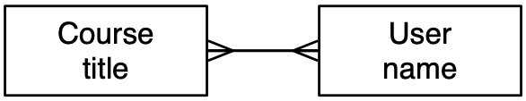
Some data relationships cannot be modeled by a simple one-to-many relationship. For example, lets say we are going to build a data model for a course management system. There will be courses, users, and rosters. A user can be on the roster for many courses and a course will have many users on its roster.

It is pretty simple to draw a many-to-many relationship as shown in Figure . We simply draw two tables and connect them with a line that has the “many” indicator on both ends of the lines. The problem is how to implement the raltionship using primary keys and foreign keys.

Before we explore how we implement many-to-many relationships, lets see if we could hack something up by extending a one-to many relationship.

A Many to Many Relationship\label{figm2m} — A Many to Many Relationship

If SQL supported the notion of arrays, we might try to define this:

CREATE TABLE Course (
    id     INTEGER PRIMARY KEY,
    title  TEXT UNIQUE
    student_ids ARRAY OF INTEGER;
);

Sadly, while this is a tempting idea, SQL does not support arrays.³

Or we could just make long string and concatenate all the User primary keys into a long string separated by commas.

CREATE TABLE Course (
    id     INTEGER PRIMARY KEY,
    title  TEXT UNIQUE
    student_ids ARRAY OF INTEGER;
);

INSERT INTO Course (title, student_ids)
VALUES( 'si311', '1,3,4,5,6,9,14');

This would be very inefficient because as the course roster grows in size and the number of courses increases it becomes quite expensive to figure out which courses have student 14 on their roster.

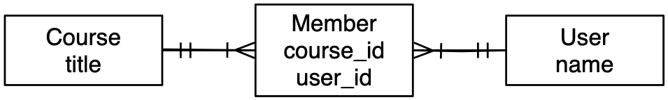
A Many to Many Connector Table\label{figm2mvrb} — A Many to Many Connector Table

Instead of either of these approaches, we model a many-to-many relationship using an additional table that we call a “junction table”, “through table”, “connector table”, or “join table” as shown in Figure . The purpose of this table is to capture the connection between a course and a student.

In a sense the table sits between the Course and User table and has a one-to-many relationship to both tables. By using an intermediate table we break a many-to-many relationship into two one-to-many relationships. Databases are very good at modeling and processing one-to-many relationships.

An example Member table would be as follows:

CREATE TABLE User (
    id     INTEGER PRIMARY KEY,
    name   TEXT UNIQUE
);

CREATE TABLE Course (
    id     INTEGER PRIMARY KEY,
    title  TEXT UNIQUE
);

CREATE TABLE Member (
    user_id     INTEGER,
    course_id   INTEGER,
    PRIMARY KEY (user_id, course_id)
);

Following our naming convention, Member.user_id and Member.course_id are foreign keys pointing at the corresponding rows in the User and Course tables. Each entry in the member table links a row in the User table to a row in the Course table by going through the Member table.

We indicate that the combination of course_id and user_id is the PRIMARY KEY for the Member table, also creating an uniqueness constraint for a course_id / user_id combination.

Now lets say we need to insert a number of students into the rosters of a number of courses. Lets assume the data comes to us in a JSON-formatted file with records like this:

[
  [ "Charley", "si110"],
  [ "Mea", "si110"],
  [ "Hattie", "si110"],
  [ "Keziah", "si110"],
  [ "Rosa", "si106"],
  [ "Mea", "si106"],
  [ "Mairin", "si106"],
  [ "Zendel", "si106"],
  [ "Honie", "si106"],
  [ "Rosa", "si106"],
...
]

We could write code as follows to read the JSON file and insert the members of each course roster into the database using the following code:

import json
import sqlite3

conn = sqlite3.connect('rosterdb.sqlite')
cur = conn.cursor()

str_data = open('roster_data_sample.json').read()
json_data = json.loads(str_data)

for entry in json_data:

    name = entry[0]
    title = entry[1]

    print((name, title))

    cur.execute('''INSERT OR IGNORE INTO User (name)
        VALUES ( ? )''', ( name, ) )
    cur.execute('SELECT id FROM User WHERE name = ? ', (name, ))
    user_id = cur.fetchone()[0]

    cur.execute('''INSERT OR IGNORE INTO Course (title)
        VALUES ( ? )''', ( title, ) )
    cur.execute('SELECT id FROM Course WHERE title = ? ', (title, ))
    course_id = cur.fetchone()[0]

    cur.execute('''INSERT OR REPLACE INTO Member
        (user_id, course_id) VALUES ( ?, ? )''',
        ( user_id, course_id ) )

    conn.commit()

Like in a previous example, we first make sure that we have an entry in the User table and know the primary key of the entry as well as an entry in the Course table and know its primary key. We use the ‘INSERT OR IGNORE’ and ‘SELECT’ pattern so our code works regardless of whether the record is in the table or not.

Our insert into the Member table is simply inserting the two integers as a new or existing row depending on the constraint to make sure we do not end up with duplicate entries in the Member table for a particular user_id / course_id combination.

To reconstruct our data across all three tables, we again use JOIN / ON to construct a SELECT query;

sqlite> SELECT * FROM Course
   ...> JOIN Member ON Course.id = Member.course_id
   ...> JOIN User ON Member.user_id = User.id;
+----+-------+---------+-----------+----+---------+
| id | title | user_id | course_id | id |  name   |
+----+-------+---------+-----------+----+---------+
| 1  | si110 | 1       | 1         | 1  | Charley |
| 1  | si110 | 2       | 1         | 2  | Mea     |
| 1  | si110 | 3       | 1         | 3  | Hattie  |
| 1  | si110 | 4       | 1         | 4  | Lyena   |
| 1  | si110 | 5       | 1         | 5  | Keziah  |
| 1  | si110 | 6       | 1         | 6  | Ellyce  |
| 1  | si110 | 7       | 1         | 7  | Thalia  |
| 1  | si110 | 8       | 1         | 8  | Meabh   |
| 2  | si106 | 2       | 2         | 2  | Mea     |
| 2  | si106 | 10      | 2         | 10 | Mairin  |
| 2  | si106 | 11      | 2         | 11 | Zendel  |
| 2  | si106 | 12      | 2         | 12 | Honie   |
| 2  | si106 | 9       | 2         | 9  | Rosa    |
+----+-------+---------+-----------+----+---------+
sqlite>

You can see the three tables from left to right - Course, Member, and User and you can see the connections between the primary keys and foreign keys in each row of output.

Modeling data at the many-to-many connection

While we have presented the “join table” as having two foreign keys making a connection between rows in two tables, this is the simplest form of a join table. It is quite common to want to add some data to the connection itself.

Continuing with our example of users, courses, and rosters to model a simple learning management system, we will also need to understand the role that each user is assigned in each course.

If we first try to solve this by adding an “instructor” flag to the User table, we will find that this does not work because a user can be a instructor in one course and a student in another course. If we add an instructor_id to the Course table it will not work because a course can have multiple instructors. And there is no one-to-many hack that can deal with the fact that the number of roles will expand into roles like Teaching Assistant or Parent.

But if we simply add a role column to the Member table - we can represent a wide range of roles, role combinations, etc.

Lets change our member table as follows:

DROP TABLE Member;

CREATE TABLE Member (
    user_id     INTEGER,
    course_id   INTEGER,
    role        INTEGER,
    PRIMARY KEY (user_id, course_id)
);

For simplicity, we will decide that zero in the role means “student” and one in the role means instructor. Lets assume our JSON data is augmented with the role as follows:

[
  [ "Charley", "si110", 1],
  [ "Mea", "si110", 0],
  [ "Hattie", "si110", 0],
  [ "Keziah", "si110", 0],
  [ "Rosa", "si106", 0],
  [ "Mea", "si106", 1],
  [ "Mairin", "si106", 0],
  [ "Zendel", "si106", 0],
  [ "Honie", "si106", 0],
  [ "Rosa", "si106", 0],
...
]

We could alter the roster.py program above to incorporate role as follows:

for entry in json_data:

    name = entry[0]
    title = entry[1]
    role = entry[2]

    ...

    cur.execute('''INSERT OR REPLACE INTO Member
        (user_id, course_id, role) VALUES ( ?, ?, ? )''',
        ( user_id, course_id, role ) )

In a real system, we would proably build a Role table and make the role column in Member a foreign key into the Role table as follows:

DROP TABLE Member;

CREATE TABLE Member (
    user_id     INTEGER,
    course_id   INTEGER,
    role_id     INTEGER,
    PRIMARY KEY (user_id, course_id, role_id)
);

CREATE TABLE Role (
    id          INTEGER PRIMARY KEY,
    name        TEXT UNIQUE
);

INSERT INTO Role (id, name) VALUES (0, 'Student');
INSERT INTO Role (id, name) VALUES (1, 'Instructor');

Notice that because we declared the id column in the Role table as a PRIMARY KEY, we could omit it in the INSERT statement. But we can also choose the id value as long as the value is not already in the id column and does not violate the implied UNIQUE constaint on primary keys.

Summary

This chapter has covered a lot of ground to give you an overview of the basics of using a database in Python. It is more complicated to write the code to use a database to store data than Python dictionaries or flat files so there is little reason to use a database unless your application truly needs the capabilities of a database. The situations where a database can be quite useful are: (1) when your application needs to make many small random updates within a large data set, (2) when your data is so large it cannot fit in a dictionary and you need to look up information repeatedly, or (3) when you have a long-running process that you want to be able to stop and restart and retain the data from one run to the next.

You can build a simple database with a single table to suit many application needs, but most problems will require several tables and links/relationships between rows in different tables. When you start making links between tables, it is important to do some thoughtful design and follow the rules of database normalization to make the best use of the database’s capabilities. Since the primary motivation for using a database is that you have a large amount of data to deal with, it is important to model your data efficiently so your programs run as fast as possible.

Debugging

One common pattern when you are developing a Python program to connect to an SQLite database will be to run a Python program and check the results using the Database Browser for SQLite. The browser allows you to quickly check to see if your program is working properly.

You must be careful because SQLite takes care to keep two programs from changing the same data at the same time. For example, if you open a database in the browser and make a change to the database and have not yet pressed the “save” button in the browser, the browser “locks” the database file and keeps any other program from accessing the file. In particular, your Python program will not be able to access the file if it is locked.

So a solution is to make sure to either close the database browser or use the File menu to close the database in the browser before you attempt to access the database from Python to avoid the problem of your Python code failing because the database is locked.

Glossary

attribute: One of the values within a tuple. More commonly called a “column” or “field”.
constraint: When we tell the database to enforce a rule on a field or a row in a table. A common constraint is to insist that there can be no duplicate values in a particular field (i.e., all the values must be unique).
cursor: A cursor allows you to execute SQL commands in a database and retrieve data from the database. A cursor is similar to a socket or file handle for network connections and files, respectively.
database browser: A piece of software that allows you to directly connect to a database and manipulate the database directly without writing a program.
foreign key: A numeric key that points to the primary key of a row in another table. Foreign keys establish relationships between rows stored in different tables.
index: Additional data that the database software maintains as rows and inserts into a table to make lookups very fast.
logical key: A key that the “outside world” uses to look up a particular row. For example in a table of user accounts, a person’s email address might be a good candidate as the logical key for the user’s data.
normalization: Designing a data model so that no data is replicated. We store each item of data at one place in the database and reference it elsewhere using a foreign key.
primary key: A numeric key assigned to each row that is used to refer to one row in a table from another table. Often the database is configured to automatically assign primary keys as rows are inserted.
relation: An area within a database that contains tuples and attributes. More typically called a “table”.
tuple: A single entry in a database table that is a set of attributes. More typically called “row”.

If you find a mistake in this book, feel free to send me a fix using Github.